AeroLap

AeroLap is a limit performance simulation tool for predicting and analysing the maximum performance of race cars and fast road cars over a defined path, typically a lap of a race track.

It has been continuously developed, and in continuous use by race teams, race car constructors and high performance road car manufacturers in a variety of categories since 1998.

AeroLap is a fully featured, professional race car lap simulator that allows you to predict the results of changes to the set-up of your car in terms of maximum performance around a fixed track time. Basic use is straightforward:

1     Set up the model of the car just as you would the real car using a series of set-up pages, one for each major module of the car. See defining the car for more details.

2     Choose a track or generate one from acquired data.

3     Click Run and watch while the simulation calculates the fastest possible theoretical lap for the car setup and track you defined.

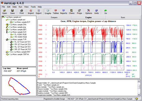
4     View the results graphically, numerically or in the report, overlaying simulated channels on data acquired from the car or on the last simulation lap.

5     Make changes to the set-up, re-run the simulation and compare the results, all in far less than the time it takes the car to run a lap on the track.

On-track performance for a flying lap is calculated with over 200 different output channels available, just like the data acquisition on the car, including some channels not possible or very difficult to measure on a car.

Using a complex, multi-layered model with many non-linear components, and performing hundreds of thousands of calculations for a run AeroLap can provide more realistic and accurate results than other methods. The results of those calculations are presented in a way that is easy to interpret, using the same skills as for the on-car acquisition. You can optionally leverage the ActiveX interface to the calculation engine to access every single property of the simulation and to automate the running of simulations, e.g. for parameter sweeps or optimisation.

The underlying calculation method is to discretise a given 3D path into small segments. For each segment the maximum thrust is applied to the car, according to the authority of the engine or braking system and limited by the grip available, driver behaviour and other forces on the car e.g. aero or gravity. A pseudo steady state solution is found for the sprung mass position and the solver focus moves to another segment. Segments are solved in the most efficient order, which is often not sequentially. When all segments have been solved the results can be presented as a continuous time history.

Back to top

 Decide race engineering strategy before going to the track.

 Prepare your setups in advance for changes in track layout, or for going to a new track.

 Make key design decisions before committing to building a prototype.

 Choose gear ratios based on their effect on laptime, automatically taking account of many factors that are not considered when using ratio charts or spreadsheet modelling such as engine performance, track gradients, ambient wind speed.

 Compare different engine torque/power curves, both in terms of predicted lap time and by plotting the engine torque or power actually being used throughout the lap.

 Run a variety of aerodynamic trims and look at lift/drag trade-offs.

 Predict ride heights and alter the suspension setup so that you are getting the best out of the car's aerodynamics.

 Examine the effect of different fuel loads on performance for pit strategy.

 Setup your suspension to get the best from the tires.

 Gain a better understanding of what affects your car's performance and why.

You can do all of this in a fraction of the time and cost it would take at the track, and you can make much better use of your track time if you have experimented with multiple set-ups before-hand.